More Outliers from the Mass–Metallicity Relation

Last week, my second paper on outliers from the mass–metallicity relation showed up on astro-ph. In the first one, which I described here, was on the low-mass high-metallicity outliers from the relation; I described in that first post more about what this so-called "mass–metallicity relation" thing actually is. We concluded in that paper that those galaxies must be running out of star-forming gas, and thus nearing the end of their star formation.

In Paper II, we are looking at the other corner of the mass–metallicity plane: massive low-metallicity galaxies. (Yes, it is easy to get tongue-tied in this game.) Most of the 42 galaxies in our sample look like this:They are very blue and what we astronomers called "disturbed." That's fancy-talk for "they've been playing rough with their neighbors and so their gas and stars have been all moved around so they look morphologically... disturbed." The key here is that simulations have shown that as galaxies interact, gas from really large scales will typically get drained into the centers of the galaxies. As it turns out, this large-scale gas will generically have a much lower metallicity than the gas originally at the galaxy center, so the large-scale gas inflow will effectively dilute the central gas. Relative to the amount of time we can expect for the star-formation to continue, it won't take very long for this new gas to get re-enriched by metals formed during the star formation itself, so we can expect for these luminous low-metallicity galaxies to be relatively rare.

In Which I Disucss What I Have Been Doing Instead Of Blogging

The astute reader has pointed out that I have not exactly been "updating" this blog lately, which is to say, I haven't posted anything in basically two months or more.

Thing is, I haven't really had much to say. I spent a week at the beach (oh, such a perfect beach it was) in June with my family and the significant other. There was sand and ocean and sky and rum and sleep and shrimp boil and sunshine everything was good. I've been reading a lot. In the last two months or so, I've re-read the entire Kushiel series (except for the middle part of Kushiel's Scion since that one isn't really all that good anyhow) in preparation for Kushiel's Mercy, which I got from the library and quickly devoured. This week I read Angelina Jolie's Notes From My Travels, which is essentially a publication of the journal she kept when beginning her work with refugees and the United Nations. (I'm particularly interested in Cambodia, and so her impressions of regions she traveled through some 4 years before me were particularly interesting, though the timing of her trip to Pakistan to see and meet Afghan refugees there in August 2001 is perhaps the trip with the most interesting timing.) I'm about halfway through Obama's Audacity of Hope; having read Al Gore's The Assault on Reason in February (which was actually the inspiration for this post, though I did at the time fully intend for a book review to be forthcoming...), I have decided to try to read more, you know, non-fiction. So far the Audacity of Hope is making me realize why so many people seem to be "in love" with Obama—he uses the word "damask" in the second paragraph of chapter 1 ... how can you not love that?! So far the book seems straightforward and honest, but then, I'm pissed off about his FISA vote and the lame-ass excuses he gave over it. I'll still be voting for him, of course—in the last eight years, McCain has gone from interesting to downright frightening—but it is good to stay informed and realistic. I also started reading Daily Kos—a totally unbiased source of information, I know, but what is? and I like the snark—which has managed to make my morning coffee-and-blogs time erm slightly longer. I also finally finished Freakonomics and The Know-It-All in May ... and I've become totally addictd to LibraryThing and its vast cataloguing and statistics-generating power. While visiting my parents, I also helped them scan in a few hundred of their books; why are such things so immensely interesting?!

Oh, yeah, and I guess I've kind of been working. The first few weeks after the beach were rough (there was a dearth of ocean, rum, and soft breezes in my office, and I'd gotten used to the 10 or more hours of sleep a night), but I had a paper accepted for publication around the end of June. I had gotten around a dozen emails about it after it first showed up on astro-ph—many of which were not just asking me to cite some obscure paper of theirs! So I think this is a case where the paper—and the interpretations—did substantially improve between revisions. So now I'm working on the "sequel" paper: paper #1 was on low-mass high-metallicity outliers from the mass–metallicity relation, so paper #2 is going to be on the high-mass low-metallicity outliers. I convinced myself today that the metallicities I'm measuring for this new sample aren't bogus, so now it's time to start compiling all of the data and building an explanation for why these galaxies are the way they are. The current plan is to present the main results at a conference in August so that some of the helpful back-and-forth that happened after the last paper showed up on astro-ph can perhaps happen before the paper is submitted this time.

I've been working on several other things as well, but getting into all of that would mean *gasp* explaining in part what my so-called "thesis" is about, and we wouldn't want to rush back into this relationship too quickly, now would we? Besides, I have a book to go read.

Paper Summary: Metal-Rich Dwarf Galaxies

Towards the last week of January, when I was hugely absorbed in trying to figure out a thesis proposal thing, a professor came into my office and started talking about the mass–metallicity relation. I knew about it, of course, but here was a new, simple idea: are the extreme outliers from this locus of galaxies real? In the spirit of a short "one month" project, it's now about three months later, and we've "finally" got a paper on said outliers on astro-ph. (I think this is a great example of: if anyone ever offers you a great idea, take it and run with it.)

So to back up a bit. What's this "mass–metallicity relation"? The short version is that a correlation exists between galaxy mass and metallicity such that the more massive a galaxy is, the more likely it is to be "metal rich." Originally this was the luminosity–metallicity relation, since how bright a galaxy is is much easier to measure than how massive it is, so on the right here I've plotted metallicity versus "absolute magnitude" in small grey points for a large sample of star-forming galaxies (remember: magnitudes are silly, so the right-hand side is brighter than the left-hand side, even though the numbers don't increase in that direction). Our outliers are, well, the larger red and green outliers from this relation; the different colors simply denote slightly different ways of selecting different subsamples. Astronomers being astronomers and not material scientists, when we say "metals" what we really mean is "any element which could not have been made in the Big Bang, i.e., basically anything not Hydrogen or Helium (or maybe Lithium but there's so little of that we'll completely ignore it)." There is of course a nice slew of caveats. The first is that the easiest way to measure the metallicity of galaxies is to limit ourselves to star-forming galaxies; all of those nice new young stars heat up the gas around them, and then as this gas cools it gives off emission lines. We can then look at the spectra of these galaxies and by measuring the how how strong various lines are relative to one another and combining it with some black magic (a.k.a. "spectral synthesis codes") we can measure the ratio of oxygen to hydrogen in a star-forming galaxy's gas. So I (and others!) basically use "metallicity" and "oxygen abundance" interchangeably, and, more precisely, I basically always mean "gas phase" abundance.

One of the interesting interchanges between theory and observation is that sometimes there will be some interesting observation (such as the obervation that galaxy mass and metallicity are correlated). So theorists will come up with a bunch of reasons why this is the case, and a few will even attempt to give explanations fo the scatter about the observed relation. A robust theory will also be able to explain seemingly strange galaxies: if a theory is able to explain why low mass galaxies have such low metallicities, then it should also be able to predict in what ways a low mass galaxy with high metallicity is different from its more mundane cousins. I spend a lot of the paper exploring various explanations (and then eliminating them) for why these galaxies could be so "weird," but I eventually hit upon one explanation which, in retrospect, is blindingly obvious.

The idea is that low mass galaxies have low metal abundances because they have low star formation rates and relatively high gas fractions (i.e., the fraction of their mass that is in gas rather than stars is large). An easy way to think of this is like so: stars turn hydrogen and helium into more massive elements (metals). As stars are formed, they the most massive ones die quickly, throwing their metal-rich selves back into the surrounding gas, thereby raising the metallicity of that gas. But a low star formation rate in a high gas fraction environment will not be making enough metals in order to fully pollute the gas around it, and so the fraction of metals in the gas will be relatively low. (This argument only really works for low-mass galaxies, but since those are the ones we're interested in, I'll ignore that subtlety for now.)

So how do you get high-metallicity low-mass galaxies? Well, presumably the galaxy would need either a very high star formation rate (so the massive stars can actually pollute the gas) or a very low gas fraction (so each supernova has a higher impact on the gas). We find that these outliers don't have unusually high star formation rates, so we conclude that they must have rather low gas fractions. But this is the same gas the stars are forming out of! So the star formation must not have very long left to go. A nice bit of supporting evidence for this scenario is the occasional mention in the literature that so-called "transition" dwarf galaxies tend to have low gas masses and higher-than-expected gas-phase metallicities; these galaxies are known as "transition" objects because they are between regular star-forming dwarfs and quiescent non-starforming dwarf galaxies. The especially neat part is that several of these galaxies have the star formation limited to their centers (like this galaxy to the left: blue in a galaxy is a sign of lots of young, recently formed stars). One way to interpret this is that star formation used to occur on all scales in this galaxy, but the gas has since been extinguished (or blown out of the galaxy) at the larger scales.

Proposing a Thesis Thing, Part the First

Sometime in November or December I started writing a blog post (most of which is included in this one, with the tenses slightly changed) on how I have to do a thesis proposal this year and what all that entails. So this is going to be a roughly five month saga compressed into a multi-post few week funfest, seeing as how there's been this Date set for April 18 or somesuch.

As I alluded to at the time, I spent several days just after Thanksgiving at a conference in Tucson. One of the ironic aspects of attending a conference on galaxy and black hole evolution is that I have done very little work which could be construed as directly relating to most of the topics discussed those three days. And yet I kept being drawn to galaxy evolution and I kept saying it is what I want to work on... The idea, I supposed, was to actually get around to doing just that.

See, I was supposed to present a "thesis proposal" in February, as the next step in this whole getting a PhD thing (the previous step being the candidacy exam last summer). (Or so was the case at the time. April is the new February, apparently.) The thought of choosing a thesis topic somewhat terrifies me, mostly because of the stereotype that choosing a thesis topic is equivalent to choosing what I'll be working on for the rest of my life. My aversion to such a decision stems from the same aversion I have to say, traditional marriage: it's not that I can't see myself working on something for the rest of my life, it's that I wouldn't want to work on one thing to the exclusion of all else.

Luckily, real life isn't a pure manifestation of stereotypes, and what a "thesis" (or, more relevantly, a "thesis proposal") should be varies from advisor to advisor. If all goes as planned, I'm essentially halfway through graduate school (or at least I was in December), which means that I will be applying for jobs in (eep!) about a year and a half. My advisor seems to think that the thesis proposal should basically be a default plan for how I am going to write enough interesting papers in that year and a half so that people will want to give me a job. In other words, it's not so much what I will be doing, but what I can do if nothing else more interesting comes along. Yet, despite the seemingly nebulous nature of said proposal, I was still somewhat freaked out over the whole thing back in November. And December. And January. Then in February and March I just kind of ignored the problem, hoping it would go away ...

Galaxies!! Part Two

Waaaaay back in June—as in, last June—I wrote a long post explaining the background, mostly about galaxies, needed to understand the work I've done on the connection between how strongly barred a galaxy is and what kind of structure its circumnuclear dust takes on. (If you want to understand the results below, I recommend reading the background post first. Also, the poster for the conference I presented this at last year can be found here.) The paper was published on December 1, and it is this paper that I will be presenting next week for the oral portion of my general exam, so I figure it's about time I get around to explaining to y'all some of the actual, you know, results.

The first step in preparing next week's talk was to re-read this paper I haven't touched in nearly a year. This has been fun, not only for the "wow! galaxies are cool!" aspect, but also because I can think things like, " 'Employ'? We employ this technique? Didn't we really just use it??" Also, all of those figures I thought were gorgeous a year ago? Turns out the font is too small on most of them, and at least one of them has a typo (as well as one table).

Our first main result was that tightly wound nuclear dust spirals are primarily found in galaxies lacking bars. This isn't all that surprising due to boundary conditions: for the dust in a circumnuclear spiral to connect to the (radial) dust lanes in a bar, the spiral must unwind somewhat, and tightly wound spirals are not somewhat unwound.

So what kinds of circumnuclear morphologies do strongly barred galaxies take on? One common feature is what we term "large grand design" (LGD) spiral structure. A LGD spiral has two prominent symmetric spiral arms which, in 90% of our LGD galaxies, distintegrate before reaching the galaxy nucleus. One frequent end for these spiral arms is at a circumnuclear starburst ring. A circumnuclear starburst ring is just what it sounds like: a ring of intense star formation and thick dust surrounding the galaxy nucleus, like the example to the right. Here, the LGD structure are the dark dust lanes on the top left and bottom right of the image, which connect onto the ring itself. Inside the ring, we see a loosely wound nuclear spiral which is distinct from the ring itself, and is likely to be "native" dust; that is, the bar is probably ineffective at funneling material to the very center of this galaxy. In our most strongly barred galaxies, those lacking LGD spirals simply have very chaotic centers (at best, a chaotic spiral), potentially with a lot of ongoing star formation.

The Lyman-alpha Forest

It seems that I am now working on the Lyman-α forest, a fair cry from stars or the Milky Way. One of the great aspects of working on the Lyman-α forest is that it relates to so many other aspects of astronomy. And, recently, it's been difficult to spend much time here and not become interested in the composition and geometry of the IGM (e.g., this and this and this).

I had heard about the Lyman-α forest for quite a while before truly understanding what it is; in this particular case, it was a picture that made all the difference.

For example, this cartoon, shamelessly borrowed from Ned Wright's page explaining the Lyman-α forest. There are three separate pieces needed to explain what is meant by the "Lyman-α forest, " or what is commonly written as the Lyα forest. First, there's the Lyman-α bit, which involves a bit about atoms and rudimentary atomic physics. Then, there's the large reservoir of gas between galaxies creatively known as the intergalactic medium, or IGM. Finally, there are the notions of redshift and thermal broadening and other fun things that can happen to change the wavelength at which a photon of light is observed.

Atoms and energy levels: As you should recall from your high school chemistry class (or as wikipedia [or here] would remind you if you were asleep that year), atoms come equipped with energy levels, and the electrons can move between the different levels. These transitions have different names, and the Lyman-α transition is the one between the n=1 and n=2 states. (Lyman-β is n=3 to n=1, Lyman-γ is 4 to 1, Lyman-δ is 5 to 1, and so on. The series of transitions into n=other states are have different names; the Lyman series is just the one named after some dude named Lyman.)

When electrons move from a higher energy level to a lower one, a photon (or two if it's a super-duper-forbidden transition) is emitted by the atom in order to conserve energy. Because the photon is carrying away the energy the atom had when it was in the excited state (i.e., when the electron was in the higher energy level), the energy the photon has is exactly equal to the energy difference between the two levels. So, when one counts the number of photons as a function of energy of some source—this is called taking a spectrum—there are certain wavelengths at which there are lots and lots of photons because lots of atoms have undergone energy transitions and emitted photons with near-identical energies. These are called emission lines.

Of course, the same thing can happen the other direction. If a photon of just the right energy encounters an atom, the atom can absorb the photon, essentially moving the electron from a lower energy level to a higher one. So if we take a spectrum of some bright source, we will see regions where a bunch of atoms have absorbed a bunch of photons all of one wavelength. These regions are known as absorption lines/features/troughs/whathaveyou.

The Intergalactic Medium (IGM): Hydrogen is by far the most common element in the universe; roughly 75% of all atoms in the universe are hydrogen atoms. Nowadays, most of the hydrogen is ionized, so instead of a proton and an electron hanging out together, they are separate. For electrons to be able to move between energy levels, it has to be associated with some nucleus, i.e., the atom has to be neutral. Even though the vast majority of hydrogen atoms in the IGM are ionized, there is enough neutral hydrogen around that Lyman-α (and other) transitions can trace the structure of the IGM. Of course, there are lots of other elements in the IGM, but we can only observe those with atomic transitions in convenient wavelength ranges; commonly observed other species are singly-ionized magnesium (MgII in spectroscopy lingo) and triply-ionized carbon (CIV).

As it turns out, the cartoon description above of the IGM as a bunch of isolated clumps of gas is wrong. A more accurate model has the gas distributed much more smoothly; the gas isn't perfectly uniform, and there are regions of low density and of high density, but the contrast between these regions is not large enough to think of the high density regions as "clouds."

Redshift, etc: The real key to being able to use absorption features to study the IGM is redshift. If we observed all of the intergalactic gas to absorb light at one wavelength, then it would be next to impossible to decipher any physical structure from a spectrum. Luckily, though, we live in an expanding universe, and so light travelling across long distances is redshifted, that is, the wavelength of a single photon gets longer as it propogates. (This is a redshift since longer wavelength means redder light.) The amount by which light is redshifted depends on the distance the light has travelled; this so-called cosmological redshift is the main thing for which Edwin Hubble is famous for figuring out. So, to return the the cartoon above, if we have some really bright faraway source, like a quasar or a gamma ray burst, then light coming towards us from this source will be redshifted. Specifically, light that was originally bluer than that of the Lyα transition will be redshifted to this wavelength, and if there is some neutral hydrogen sitting around where this happens, then it will be able to absorb that light. The more neutral hydrogen (i.e., the higher the neutral hydrogen density) at a given location, then the more Lyα light that will be absorbed. There is a lot of hydrogen in the universe, and the universe is really big, so spectra wind up looking more like this than the above cartoon:
The big peak on the right is due to Lyα emission from the quasar itself, and all the mess to the left (bluewards) of that is the Lyα forest. Lots and lots of absorption.

If this was the end of the story, then it would be fairly easy to go from a map of absorbed light to a density map of the IGM along some line of sight. Alas, this is astronomy, so there are lots of extra things going on. The first is that the gas in the IGM isn't perfectly cold; it has some temperature and so the atoms are moving around relative to one another, which causes individual lines to be smeared out. Observationally, this isn't all bad: we astronomers like knowing about temperatures as well as densities—and the relationship between the two.

As I mentioned earlier, astronomers now know that the IGM does not consist of discrete clouds floating around in a vast emptiness; the gas density instead fluctuates about some constant value. Part of what I am working on now is to try to determine what sets the scale of these fluctuations, or, equivalently, what sets the scale on which the IGM and the Lyα forest are smooth.

Variable Stars Near the Galactic Center

I'll try to make it through this post without making any snide or snarky remarks about how boring stars are and how they're really just point particles and how caring about any one in particular is just stamp collecting.

Whoops.

So apparently the majority of the papers I have first authored at this point in my career are about stars. I've even published an entire paper on just two stars (or one, depending on how you count ... the idea that "a binary star" is really two stars hasn't fully infiltrated the nomenclature, it seems). It took a lot of doing while writing this paper to figure out just why anyone would care about a bunch of variable stars; for the paper I wrote about dust structures at other galactic center, the explanation of why the topic is interesting was much easier to sink my teeth into (though "centers of galaxies are interesting because I get to look at pretty galaxies" is apparently not a sound argument).

This paper is about "variable stars near the Galactic center," where "near" is defined as within about 2 pc (about 6.5 lightyears) of the supermassive black hole, Sgr A*, at the Milky Way's center. I've put a completely gratuitous picture of the field below; the yellow X marks where Sgr A* is, the dots are on variable stars, and the cyan dots are the stars I actually talk about in the paper. The bar denoting how much 30'' is corresponds to 3.6 lightyears. This field of view (i.e., how much we can see) is larger than many of the stellar variability studies near the Galactic center, but still small enough that we can basically assume that all of the stars we are looking at are pretty close to Sgr A*. The metric I usually keep in mind is that the size of a resolution element when looking at nearby galaxies with the Hubble Space Telescope is 1–15 pc. In other words, this entire field of view would look like just a few bright pixels if it were in another galaxy.

Or, it would look like a few dark pixels, if we were looking at the galaxy edge on. And, because we are in the disk of the Milky Way, we are looking at the Milky Way edge on. This is why things like exactly where the center of the Galaxy is and the fact that the Milky Way is a barred galaxy weren't known until recently. Spiral galaxies like the Milky Way have lots of gas and dust in them between all of the stars (so it is called the "interstellar medium," or ISM). This dust absorbs light, so it is very difficult to see stars near the center of the Galaxy (which is thought to be about 7600 pc away these days). Because dust absorbs more blue light than red light, something sitting behind a whole bunch of dust looks redder than it intrinsically is. This is why absorption due to dust is referred to as "reddening," and why we have to look at infrared wavelengths to be able to see stars near the Galactic center.


The paper is essentially just a list of the 110 variable stars we identified; about 90 of these are new (depending on how you count). "Look, here's a list of variable stars and their light curves" doesn't make for all that interesting a paper—even if most of the list is new—so I put a decent amount of effort into trying to cross-correlate our catalog with known sources (known variable stars, of course, but also X-ray and radio catalogs) at the Galactic center. Many of our variables that matched up to other sources are fairly well-known, and even have names. One of these stars was IRS 16SW, which we wrote a paper on last fall, but I think the most interesting of the previously-known objects in our catalog is IRS 10*. This is our light curve for IRS 10*; the vertical axis is the K-band magnitude (remember, smaller numbers means brighter!) and the horizontal axis is in days. What makes this object actually interesting isn't that its brightness changed so much, but that by poking around in the literature (literally—remember that big pile of papers?), I found that there are several stellar masers and a bright X-ray source sitting at pretty much the same location. When I started this project, I definitely didn't know anything about masers, so here's pretty much all you need to know: (1) they are like lasers, except at radio frequencies, and they actually amplify light instead of merely letting it coherently oscillate; and (2) masers associated with stars are generally associated with stars with lots of gunk around them (the stuff actually doing the masing); these stars are usually "asymptotic giant branch" (AGB) stars, which are basically old stars that are busy shedding their outer envelopes. The idea that IRS 10* is an AGB star isn't all that exciting; what is exciting is that AGB stars are not bright X-ray sources, so if the nearby X-ray source actually is associated with IRS 10*, then it probably means that IRS 10* has some dead companion (like a white dwarf) which is accreting mass from the AGB star. (If the X-ray source isn't associated with IRS 10*, the question then becomes: what can cause such a bright X-ray flux and not vary at these wavelengths?)

When astronomers hear about a new catalog of variable stars, the first thing they almost always ask is, "how many periodics?" I spend a lot of time in the paper talking about two "enigmatic" variables with periods of about 42 days; basically after a page or so of babble I get around to saying we don't know what the hell these things are, except that they're interesting and we'd like to know, and that someone needs to try to take more data to figure out what they are. These are their light curves to the left; H and K are the names of the two filters our data are in. (When people started naming their filters back in the day, they gave them sensible names like "b" for the one that let through blue light and "r" for the one that let through red light. The filter just redder of the r-band filter is "i," for infrared, so when the filters started getting further into the infrared they just kept going to j, H, K, L, etc. So K band is redder than H band. And, please, don't think too hard about how the alphabet works right there.) The left-hand panels of the light curves are in days, like the light curve of IRS 10* above; the right-hand panels are phased according the period P so you can see what the light curve is "really" doing.


And just to completely fulfill the promise of this post's title, here are some of my favorite (read: prettiest) light curves from the paper ... for all of these, K band is on top and H band is on the bottom and such, just like before...

Spring!

Well, spring has officially been here in the northern hemisphere for several days now, and now that I attend a school whose terms align accurately with the seasons, this also means that spring quarter will be starting Monday. The ice and snow are being replaced with more savory things, like flowers and pollen and ants, and apparently our office building isn't going to have the air conditioning ("cooling systems") turned on until April 10, so it'll be like going to a tropical non-breezy treeless forest every day.

Now, the most important aspect to remember about this upcoming quarter is that I will be taking my Last. Class. Ever. Sure, there might be some set of exams I'll have to take at the end of the quarter, and they're probably going to even give me another degree, but such things are inconsequential when we consider the raw facts of no more classes. See, classes and I, we just don't get along. I'm not a big fan of sitting still for extended periods of time, let alone having time taken out of the middle of my day for sitting still. We used to be pretty close: I took classes and they gave me good grades and everything was hunky-dory. Then in 10th grade it happened: I did my first research project. I had a couple of magenta liquid crystal cells I hooked up to a battery and some switches, and I spent hours and hours heating them up and freezing them (my first fun with dry ice) and watching how the impurities in the material affected the phase transitions. I was hooked. What's the point of taking classes when I could be having fun instead? So for the last nine years (yrrgh! that long??) I've been rather impatiently waiting until I could quit wasting my time on all these silly sit-and-take-notes and then do-these-everso-enlightening-problems classes, and start doing real science.

And when I put it that way, I'm not quite sure I've entirely internalized just how exciting this is going to be.

Peanut Star

If this star weren't already named "GCIRS 16SW," I would christen it the Peanut Star. Like a peanut, this star has two nuclei (technically, individual stars, but for some reason astronomers say that the two stars in a binary system form a (single) binary star). The two stars are really really close to one another; so close, in fact, that they share material and have a "common envelope," which you can think of as the peanut's shell. Oh, and they're really big: each one is about 50 times as massive as the Sun with a radius about 60 times as large as the Sun's radius. That's freaking huge, by the way. (The axes in this model on the right are in units of the radius of the Sun.) You can count on one hand (without even resorting to counting in binary) the known number of stars in binary systems with comparable masses.

The aspect of this particular star system that makes it so interesting is the "GC" in "GCIRS 16SW." GC stands for Galactic center; specifically, our Peanut Star is only about a fifth of a light year (that's about 12,000 times the distance from the Earth to the Sun) away from the massive black hole, Sagitarius A*, at the center of the Milky Way. (In the picture on the left, the yellow arrows are pointing at Sgr A*, and the green arrow is pointing at IRS16SW.) For comparison, the star nearest our own Sun is about 4.2 light years away. While there is a lot of other evidence for really massive stars near the Galactic center, astronomers still don't know exactly how they got there. Massive stars don't live for very long, which means that either they were born frighteningly close to the big black hole, or they were born slightly further away and somehow got transported really close in very quickly. The problem with these stars being born so close to the black hole itself is that stars are usually born in a cloud of cold gas: the gas has to be cold so that it will collapse and get dense enough to form stars. But the gas near the black hole is moving really fast: it's not cold! Lots of ideas trying to solve this dilemma have been put forward, but so far, there isn't one terribly convincing explanation.

By the way, the short paper all about this object that I've been working on recently showed up on astro-ph today.

Weak Lensing

All of the (physics) research I did as an undergrad related in some way to gravitational lensing. As papers with long author lists often take a while to go through the do-the-work-then-do-more-work-then-someone-writes-it-up-then-argue-over-what-got-written-up-then-try-to-publish-it process, it's no big surprise that a paper on "high precision weak lensing analyses" based in part on work I haven't touched in two years now showed up on astro-ph this week.

Gravitational lensing refers to the bending of the path of light due to gravity. If there is mass between us and some faraway source (which for something sufficiently far away, there always is) then that mass will act as a lens and distort how the source appears to us. If the source is very close to directly behind the lens, the source's image can be so distorted that a single galaxy is stretched out into an arc, or even have multiple images. This is known as strong lensing. In weak lensing, the background image is only slightly distorted; for instance, a perfect circle might be sheared to appear slightly elliptical. The neat—and useful—thing about gravitational lensing is that it is only susceptible to where the mass is—and that's it. Even if we can't "see" the mass. The other incredibly alluring aspect to graviational lensing is its (albeit, somewhat superficial) simplicity: all we need is a working theory of gravity. That's it. One theory. No chemistry, no convection modelling, no particle physics, no theory of galaxy evolution or anything else of the like.

We define the "ellipticity" of an object to be (1 - b/a), where b/a is the axis ratio. (If it's a circle, for instance, then the long axis and the short axis are the same length (the diameter), so a circle has zero ellipticity. A straight line, on the other hand, has an ellipticity of 1.) The effects of weak lensing are very very small—only on the order of a few percent—and since a typical galaxy has an ellipticity of tens of percent, it's impossible to measure distortions due to weak lensing for a single galaxy.

This doesn't stop us, however, from measuring the effects of weak lensing on lots of galaxies. Specifically, lensing doesn't happen haphazardly; the direction along which a galaxy is sheared tells us about where the mass is that is doing the lensing. The idea is that if you have some field of un-lensed galaxies, then they should be randomly oriented, and have an average shear of zero. On the other hand, say we have some lensing mass (like a cluster of galaxies) then the average shear of the background galaxies is not zero, and we can figure out how the mass is distributed in the cluster.

Now, this sounds all fine and dandy, but there are two very difficult steps. The obvious one is that "measuring the shear" of a galaxy isn't exactly the most straightforward procedure. Sure, you can just measure the axis ratio, but unfortunately, it's not nearly that simple. Galaxies are very complicated creatures, and deconvolving the galaxy's inherent properties from the changes due to lensing is... tricky. Is it better to directly measure the shape moments of the galaxy, or do you take an idealized model of a galaxy and stretch and squish it until it looks like the one in question? We don't really know.

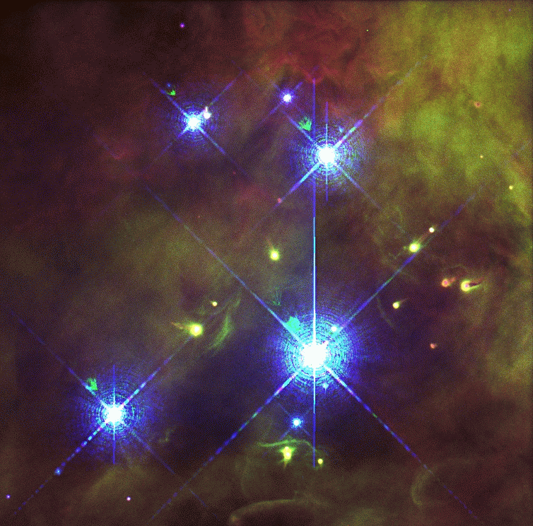
The much more subtle problem is that of the PSF, or point spread function. See, data have this unfortunate feature of not being ideal. The PSF is one of the descriptions of how data can be annoying; it describes how a single point of light is spread out into a blob. When you see spikes on images, for instance, they are due to the PSF. The irritating part is that the PSF often has an ellipticity on the order of a few percent (just like the shear signal we want to measure!), varies with time (so not all of your images have the same PSF), and can vary across the detector itself (so that the PSF on the left-hand side of the image is different from on the right-hand side). The PSF must be accounted for before the shear can be measured, and a mis-estimation in the PSF's properties can lead to a mis-measurement of the shear signal. And then, assuming the PSF is perfectly modelled (unlikely), is it better to just subtract the PSF's ellipticity from that of the galaxies, or should we attempt to deconvolve the galaxy and the PSF? Again, there are arguments both ways, but no clear answer.

This recent work is part of a courageous attempt to try to determine which measurement methods work, which don't, and, more importantly, why. This is perhaps more effective than the scientific equivalent of lots of people saying, "mine's better than yours because I like mine and I don't like yours." What we have done is to make a set of simulated images, with realistic PSFs, realistic galaxies, and realistic noise, like what one would get from data taken at a large ground-based telescope. Most importantly, a shear was applied to each image which could then be measured. (My contribution to this work, by the way, was in making the simulated images.) Different people threw their weak lensing analysis pipelines at the images just like they would real data, and from their results, we can now quantitatively talk about why a certain method is more effective at correcting for the PSF than another method, or in what situations certain methods are more or less effective at measuring the shear. Other factors potentially affecting shear measurment, such as how galaxy evolution and—get this—pixel size, are also becoming clearer. The cautionary bit is that anyone doing or planning on doing a weak lensing survey should strongly test their measurements methods on simulated data. The good news, though, is that "high precision" weak lensing is in fact possible.

Dots

I can't remember the last time I felt like everything in my life was simply going well. It's a strange and wonderful feeling. I highly recommend it.

Anyhow, seeing as how my paper was accepted by ApJ (the Astrophysical Journal) last night, I might as well start babbling about my next project with Kris Stanek.

The main goal of this project is to have something short, sweet, and fun, from which I can learn a lot and publish a paper. There are some near-infrared data lying around from 2000 through 2002 that some guys in our department took in order to look at one object, but they never got around to analyzing the rest of the data. So, we've got a bunch of images of the center of the Milky Way, and now we can look for variable sources, such as binary stars or pulsating stars or other crazy things. One of the exciting things about the cluster of stars at the center of the Galaxy is that there are both old and young stars (which is unusual---usually all of the stars in a cluster are the same age) and so there can be a lot of crazy stuff going on.

The way we are looking for variable stars is with a method called image subtraction. It's totally nuts that this works; we can often get fairly good light curves (graphs of how the brightness changes with time) of stars in regions so crowded that we can't even resolve the individual stars. To do this, we first make a reference image from some of the really good looking images in the set, and then subtract all of the other images from the reference (hence image subtraction). Stars that don't change in brightness ("vary") as time passes from image to image don't show up in the subtracted images, but ones whose brightnesses change do show up. We then, with the help of some black magic and code, can plot the light curves of the stars in the field.

Then comes the fun part. Lots of variable stars vary with some period; for instance, an eclipsing binary varies according to how long it takes for the two stars to go around one another. So, we just plop the data into a program and fiddle with it. This is what I spent this afternoon playing with. It's like connect-the-dots on steroids. The really fun part of it is playing with the phase-modulator, which folds the lightcurve up according to some phase, which I then get to futz around with.

The current plan is to have lightcurves for all of the sources in the field by tomorrow, or maybe Thursday. Not bad considering we started yesterday morning ...

And then I get to spend a month tweaking all sorts of parameters and redoing everything many many times and looking at lightcurves all squinty-eyed until I don't know left from right (I already don't know up from down) and we have everything all set. And much to Kris's chagrin, I don't think we'll actually have the paper finished by next Friday ...

Galaxies, background

I've finally arrived in Ishigaki. There is time set aside for a poster session today, and since I got bored on the plane yesterday and already wrote this up, I think I'll just give you some background on the research I've spent the last 9 months doing. Results to come later! The paper is at astro-ph/0606460.

First, a bit of background. To fully appreciate this project, you have to understand that galaxies are cool. Like, sexy cool. Like, really really pretty. Specifically, spiral galaxies are just to die for. Just look at any of the pictures I have here and you'll understand what I mean. One reason galaxies are so awesome is that they have a lot of stuff in them: stars, large groups of stars (called star clusters), gas (like H₂, CO, etc.), and dust (tiny grains of stuff, like dust on Earth, but without all of the dead skin cells). There is a lot more gas than dust, but usually where there is dust, there is gas, and as dust absorbs and scatters more light than the gas, it is easier to observe where the dust is and infer that there's a bunch of gas there as well. It's interesting to know where the gas is because if you get a bunch of gas into a small region, then stars begin to form. Oh, and it's pretty.

Now that that's out of the way, you should also know that most galaxies are barred. This means that instead of just a mess of spiral arms, there is some straight feature in the middle, such as is seen in NGC1300 or NGC1530. Bars are believed to funnel gas and dust from the outer regions of galaxies to the centers. It has been observed that, in general, barred galaxies have a higher concentration of gas at their centers than unbarred galaxies do, which is a bit of evidence that the bar is responsible for transporting the gas to the center. What we tried to investigate in this project is exactly what happens to the structure or morphology of the gas (or, more specifically, the dust) when it gets near the center.

We made these things called "structure maps" in order to look at where the dust is (all of the grayscale images in the paper and on the poster are structure maps). The dark regions are due to dust, while the bright regions are due to emission (which usually indicates star formation). These were made from archival HST (Hubble Space Telescope) data. HST is really good about making data publicly available after a short time; anyone can easily search their archive and download the data. There were a few papers published which had measured barstrengths for a bunch of nearby galaxies, and using this list I searched for which galaxies have available HST data including the galaxy center. I then downloaded these, ran some code on the files, and created the structure maps.

Once all of the structure maps were made, we finally got to look at all of the galaxies. We classified the central regions into six different categories. It's been known for a while that spiral galaxies often have nuclear spirals. Large-scale spirals are usually made of young, blue stars, and are essentially the size of the galaxy---on the scale of ten parsecs, say. (One parsec is the distance at which one AU (the distance from the Earth to the Sun) subtends one arcsecond on the sky. It's a little over 3 lightyears.) Nuclear spirals are completely distinct from these large-scale spirals; they are regions of slightly higher gas and dust density, are typically less than one kiloparsec in size. Our nuclear morphology classification scheme has four categories for nuclear spirals: grand design (GD), loosely wound (LW), tightly wound (TW), and chaotic spiral (CS). The grand design class is based on large-scale grand design spirals: there are two prominent symmetric arms which, for our definition, are seen to extend into the galaxy nucleus. This is an interesting class because it has been observed (and theorized) that GD structure should be found primarily in barred galaxies; dust lanes along the bar are seen to spiral towards the nucleus once they reach the central regions. LW and TW spirals are basically just coherent spirals, but the tightly wound ones are, well, more tightly wound. (The prototypes figure has a good visual example of the difference between these two classes.) How tight the spiral is can tell us a lot about the environment in which the spiral was formed and exists. Chaotic spirals are nuclear spirals that, while still having a unique sense of chirality, are relatively incoherent. The other two classes, chaotic (C) and no structure (N) are for nuclear regions with no clearly discernible spiral structure.